Stage 3: Counterfactual prediction
In this tutorial, we will walk through how to use the CASCADE model trained in stage 2 to conduct counterfactual inference.
[1]:
import anndata as ad
import networkx as nx
import numpy as np
import scanpy as sc
import seaborn as sns

from cascade.data import configure_dataset, encode_regime, get_configuration
from cascade.graph import annotate_explanation, core_explanation_graph, prep_cytoscape
from cascade.model import CASCADE
from cascade.plot import set_figure_params
[2]:
set_figure_params()
Read data and model
[3]:
adata = sc.read_h5ad("adata.h5ad")
[4]:
cascade = CASCADE.load("tune.pt")
[5]:
scaffold = nx.read_gml("scaffold.gml.gz")
graph = nx.read_gml("discover.gml.gz")
Specify counterfactual condition
Suppose we want to predict the counterfactual effect of triple gene perturbation "CEBPB,KLF1,MAPK1" for the negative control cells, we’ll need to first extract some control cells, and then specify the perturbation in a column in adata.obs (e.g., "my_pert"), in the same comma-separated format as the "knockup" column:
[6]:
ctrl = adata[adata.obs["knockup"] == ""]
sc.pp.subsample(ctrl, n_obs=1000)
ctrl.obs["my_pert"] = "CEBPB,KLF1,MAPK1"
Then we call encode_regime again to encode this counterfactual perturbation into a binary regime matrix, here in a new layer called "ctfact":
[7]:
encode_regime(ctrl, "ctfact", key="my_pert")
We’d also need to call configure_dataset again to let the model use this new regime:
[8]:
configure_dataset(ctrl, use_regime="ctfact")
get_configuration(ctrl)
22:30:46.858 | WARNING | 1633490:data:configure_dataset - Overwriting existing `regime` = "interv".
[8]:
{'covariate': 'covariate',
 'layer': 'counts',
 'regime': 'ctfact',
 'size': 'ncounts'}
Run counterfactual prediction
Now we use the counterfactual method to perform counterfactual prediction with this newly specified perturbation:
[9]:
ctfact = cascade.counterfactual(ctrl, sample=True)
22:30:46.885 | INFO     | 1633490:utils:autodevice - Using GPU [3] as computation device.
22:30:47.051 | INFO     | 1633490:core:predict_mode - Number of topological generations: [68, 88, 70, 101]
Here we specified sample=True to make the model output random samples from the counterfactual negative binomial distribution, which would better represent the distribution than a simple mean.
The prediction will be saved in both ctfact.X and ctfact.layers["X_ctfact"], where ctfact.X is the average prediction across SVGD particles, and ctfact.layers["X_ctfact"] contains the per-particle predictions with shape (n_obs, n_vars, n_particles). Note that both of these are in raw count scale.
[10]:
ctfact.X
[10]:
array([[  0.  ,   6.5 ,  16.5 , ...,   0.  ,   0.  ,  72.25],
       [  1.  ,  10.5 ,  23.25, ...,   0.  ,   0.  , 140.  ],
       [  0.  ,  11.75,  32.75, ...,   0.  ,   0.  , 157.5 ],
       ...,
       [  0.25,   6.  ,  19.5 , ...,   0.  ,   0.  ,  59.25],
       [  0.25,   9.  ,  19.5 , ...,   0.  ,   0.  ,  90.75],
       [  0.5 ,   4.5 ,  18.  , ...,   0.  ,   0.  ,  77.25]],
      dtype=float32)
[11]:
ctfact.layers["X_ctfact"].shape
[11]:
(1000, 1064, 4)
For counterfactual prediction of CASCADE designs, you would also need to specify the
designargument to thecounterfactualmethod.
Please visit the documentation of counterfactual for more details.
The same can also be achieved using the command line interface, with the following command:
cascade counterfactual -d ctrl.h5ad -m tune.pt -p ctfact.h5ad [other options]
Counterfactual differential expression comparison
To check for counterfactual effects, we are expected to compare the predicted dataset (ctfact) with the input dataset (ctrl). However, to avoid artifacts caused by model prediction biases, it is recommended to compare the predicted dataset (ctfact) with a “nil prediction”, i.e., model prediction with the original perturbation labels.
Here, we can go back to use the "interv" regime to obtain the “nil prediction”:
[12]:
configure_dataset(ctrl, use_regime="interv")
get_configuration(ctrl)
22:30:49.596 | WARNING | 1633490:data:configure_dataset - Overwriting existing `regime` = "ctfact".
[12]:
{'covariate': 'covariate',
 'layer': 'counts',
 'regime': 'interv',
 'size': 'ncounts'}
[13]:
nil = cascade.counterfactual(ctrl, sample=True)
22:30:49.790 | INFO | 1633490:core:predict_mode - Number of topological generations: [68, 88, 70, 101]
Now we combine and log-normalize both predictions to perform differential expression analysis:
[14]:
combined = ad.concat({"nil": nil, "ctfact": ctfact}, label="role", index_unique="-")
combined.X = np.log1p(combined.X * (1e4 / combined.obs[["ncounts"]].to_numpy()))
combined
[14]:
AnnData object with n_obs × n_vars = 2000 × 1064
    obs: 'guide_id', 'gemgroup', 'ncounts', 'knockup', 'my_pert', 'role'
    obsm: 'X_pca', 'covariate'
    layers: 'counts', 'interv', 'ctfact', 'X_ctfact'
[15]:
sc.tl.rank_genes_groups(combined, "role", reference="nil", rankby_abs=True, pts=True)
de_df = sc.get.rank_genes_groups_df(combined, "ctfact").query("pct_nz_group > 0.05")
de_df["-logfdr"] = -np.log10(de_df["pvals_adj"]).clip(lower=-350)
de_df.head()
/rd1/user/caozj/CASCADE/conda/lib/python3.11/site-packages/pandas/core/arraylike.py:399: RuntimeWarning: divide by zero encountered in log10
  result = getattr(ufunc, method)(*inputs, **kwargs)
[15]:
| names | scores | logfoldchanges | pvals | pvals_adj | pct_nz_group | -logfdr | |
|---|---|---|---|---|---|---|---|
| 0 | KLF1 | 207.035004 | 1.951955 | 0.0 | 0.0 | 1.0 | 350.0 |
| 1 | PNMT | 171.383087 | 2.364175 | 0.0 | 0.0 | 1.0 | 350.0 |
| 2 | CEBPB | 152.714493 | 2.131128 | 0.0 | 0.0 | 1.0 | 350.0 |
| 3 | TMSB10 | 144.004883 | 1.232379 | 0.0 | 0.0 | 1.0 | 350.0 |
| 4 | MAPK1 | 134.214584 | 1.047204 | 0.0 | 0.0 | 1.0 | 350.0 |
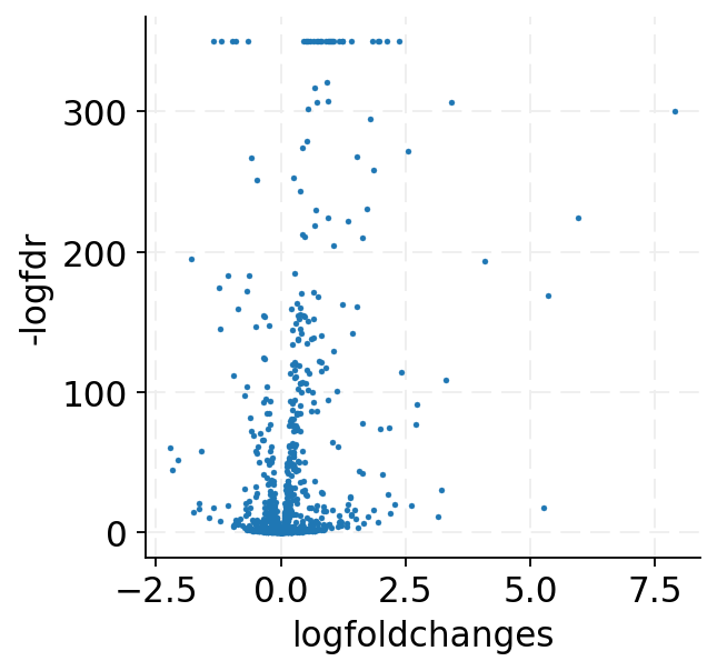
[16]:
ax = sns.scatterplot(data=de_df, x="logfoldchanges", y="-logfdr", edgecolor=None, s=5)
Explain counterfactual prediction
To understand why CASCADE made the above prediction, we can use the explain method to decompose the contribution into individual components in the model.
The method needs both a factual dataset (ctrl) and a counterfactual prediction (ctfact), properly configured as below:
[17]:
configure_dataset(ctrl, use_regime="interv")
get_configuration(ctrl)
[17]:
{'covariate': 'covariate',
 'layer': 'counts',
 'regime': 'interv',
 'size': 'ncounts'}
[18]:
configure_dataset(ctfact, use_layer="X_ctfact")
get_configuration(ctfact)
22:30:52.161 | WARNING | 1633490:data:configure_dataset - Overwriting existing `layer` = "counts".
[18]:
{'covariate': 'covariate',
 'layer': 'X_ctfact',
 'regime': 'ctfact',
 'size': 'ncounts'}
[19]:
explanation = cascade.explain(ctrl, ctfact)
explanation
[19]:
AnnData object with n_obs × n_vars = 1000 × 1064
    obs: 'guide_id', 'gemgroup', 'ncounts', 'knockup', 'my_pert'
    var: 'perturbed', 'highly_variable', 'highly_variable_rank', 'means', 'variances', 'variances_norm', 'selected'
    uns: '__CASCADE__', 'hvg', 'log1p', 'pca'
    obsm: 'X_pca', 'covariate'
    varm: 'PCs'
    layers: 'counts', 'interv', 'ctfact', 'X_ctfact', 'X_nil', 'X_ctrb_i', 'X_ctrb_s', 'X_ctrb_z', 'X_ctrb_ptr', 'X_tot'
The explanation is also an AnnData dataset with predictions from individual model components saved in separate layers.
We can pass this explanation dataset to the annotate_explanation function to annotate the contributions on graph nodes and edges:
[20]:
explanation_graph = annotate_explanation(
    graph, explanation, cascade.export_causal_map()
)
explanation_graph.number_of_nodes(), explanation_graph.number_of_edges()
[20]:
(1064, 12294)
Note that annotate_explanation has a cutoff argument (by default 0.2) that you may want to adjust, which specifies an cutoff of predicted effect (in log-normalized expression space), below which the effect is deemed too small to explain.
We can then extract a core subgraph that explains expression changes for a specific list of genes (e.g., top 10 genes with the most prominent changes), using the core_explanation_graph function:
[21]:
response = de_df["names"].head(20).to_list()
response
[21]:
['KLF1',
 'PNMT',
 'CEBPB',
 'TMSB10',
 'MAPK1',
 'S100A11',
 'ISG15',
 'SH3BGRL3',
 'FCER1G',
 'S100A10',
 'GMFG',
 'IL2RG',
 'PIM1',
 'NPW',
 'BLVRB',
 'ACTB',
 'EMP3',
 'NTRK1',
 'LGALS1',
 'RELN']
[22]:
core_subgraph = core_explanation_graph(explanation_graph, response)
core_subgraph.number_of_nodes(), core_subgraph.number_of_edges()
[22]:
(50, 107)
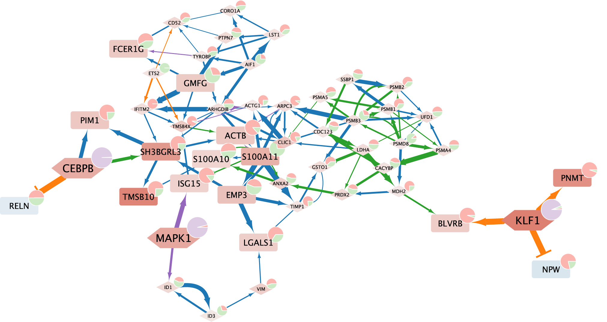
This core subgraph can be exported to Cytoscape for visualization using the utility function prep_cytoscape:
[23]:
nx.write_gml(
    prep_cytoscape(core_subgraph, scaffold, ["CEBPB", "KLF1", "MAPK1"], response),
    "cytoscape.gml",
)
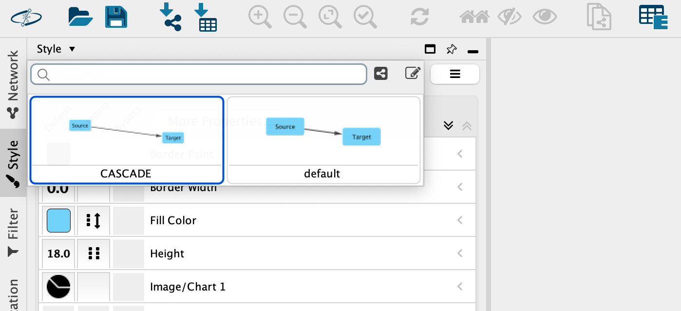
You may download a template Cytoscape file containing corresponding styles from:
Click here to apply style:
Below is an example visualization of the above core explanation graph: